Disclaimer: This is part of my notes on AI research papers. I do this to learn and communicate what I understand. Feel free to comment if you have any suggestion, that would be very much appreciated.
This month a new topic hit AI community. A new proposal to find an alternative to Multi-Layer Perceptrons (MLPs) was unleashed, leading to a heavy discussion in social media. Although authors claim that Kolmogorov-Arnold Networks (KANs), the experiments that provide the empirical evidence fall short in complexity. This, together with the massive reaction an hype, has triggered many academics to be sceptical about the promising capabilities of KANs. But what are KANs?
In order to get my own understanding of the topic I would like to read the original paper, as well as other people proposals, derived literature and the mathematics behind, such as the Kolmogorov-Arnold Representation Theorem, and how community is reacting to this new proposal.
The following post is a deep dive on the paper KAN: Kolmogorov-Arnold Networks by Ziming Liu, Yixuan Wang, Sachin Vaidya, Fabian Ruehle, James Halverson, Marin Soljačić, Thomas Y. Hou and Max Tegmark, from California Institute of Technology, Northeastern University, Massachusetts Institute of Technology, and The NSF AI Institute for Artificial Intelligence and Fundamental Interactions.
In this paper authors provide extensive numerical experiments to show that KANs can lead to remarkable accuracy and interpretability improvement over MLPs.
Introduction
MLPs, which are fully-connected feedforward neural networks, are the foundational building block’s of modern deep learning. However, since there is a trend for increasing the size of models, the following question rises: Are MLPs the best and most scalable non-linear regressors we can build? Authors propose KANs as a promising alternative to MLPs that tackle this question.
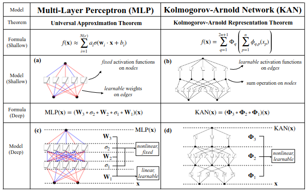
In machine learning we want to approximate (learn) parameterized functions (models) to infere something from a given dataset. MLPs are inspired by the Univesal Approximation Theorem (UAT), which states that any continuous function can be approximated by an MLP. Formally:
UAT: Let $C(X,\mathbb{R}^m)$ denote the set of continuous functions from $X \subset \mathbb{R}^n$ to $\mathbb{R}^m$. Let $\sigma \in C(\mathbb{R},\mathbb{R}^n)$. Then $\sigma$ is not polinomial if and only if for every $n\in \mathbb{N}$, $m\in\mathbb{N}$, $K\subseteq \mathbb{R}^n$ compact, $f\in C(K, \mathbb{R}^m)$ and $\epsilon > 0$, there exists $k\in\mathbb{N}$, $A\in\mathbb{R}^{k\times n}$, $b \in \mathbb{R}^k$, $C \in \mathbb{R}^{m \times k}$ such that $$ \sup_{\textbf{x}\in K} ||f(\textbf{x})-g(\textbf{x})||<\epsilon $$ where $g(\textbf{x}) = C \cdot (\sigma \circ(A \cdot \textbf{x} + b)).$
Proof of UAT
Therefore, theoretically, a sufficiently large MLP should be able to fulfill our machine learning needs.
Kolmogorov-Arnold Networks
Conversely, KANs are inspired by a representation theorem, that is Kolmogorov-Arnold Representation Theorem (KRT). Formally:
KRT: Let $C([0,1]^n,\mathbb{R})$ denote the set of continuous functions from $[0,1]^n \subset \mathbb{R}$ to $\mathbb{R}$. Therefore, if $f \in C([0,1]^n,\mathbb{R})$, then $f$ can be written as a finite composition of continuous functions of a single variable and the binary operation of addition. That is: $$ f(\textbf{x}) = f(x_1, \dots, x_n) = \sum_{q=0}^{2n+1}\phi_q\bigg( \sum_{p=1}^n \psi_{q,p}(x_p) \bigg). $$ Where $\phi_q: \mathbb{R} \rightarrow \mathbb{R}$ and $\psi_{q,p}:[0,1] \rightarrow \mathbb{R}$ are continuous functions.
Proof of KRT
In this sense, the theorem shows that the only true multivariate function is the sum, since any other function can be represented as a sum of univariate functions. KANs exploit this theorem to build a new type of model that approximates functions by learning the univariate functions $\phi_q$ and $\psi_{q,p}$. However, the theorem is not directly applicable to machine learning since it only demands for continutity, not differentiability. In practice, sometimes $\phi_q$ and $\psi_{q,p}$ are not differentiable, and can be even fractal, difficulting the optimization process.
Authors propose going beyond the equation of KRT and generalize it to allow for arbitrary width and depth. Not stick with two layers and the $2n+1$ terms. They claim this allows the model to find smoother non-linearities and better approximations.
Like MLPs, KANs also have fully-connected structures. However, while MLPs place fixed activation functions on nodes, KANs’ activation functions are learnable. Thus, KANs have no linear weight matrices, instead each weight parameter is replaced by a learnable 1D function parameterized as a spline.
Despite the elegant mathematical interpretation, authors advise that KANs are nothing more than combinations of splines and MLPs, leveraging their respective strengths and avoiding their weaknesses.
| Strengths | Weaknesses | |
|---|---|---|
| Splines | Accurate for low-dimensional functions, easy to adjust locally, able to switch between different resolutions | Huge curse of dimensionality problem |
| MLPs | Less curse of dimensionality | Less accurate than splines in low dimensions |
KAN Architecture
As KRT states, KANs are built by composing univariate functions, which are approximated by B-splines.
A B-spline or basis spline, is a spline function that has minimal support with respect to a given degree, smoothness, and domain partition. A spline is a piecewise polynomial function that is continuous and has continuous derivatives up to a certain order at the boundaries of each piece,
(INCLUDE SPLINE DEFINITION AND EXAMPLES)
They define the KAN layer as a matrix of $1D$ functions $$ \Phi = \{\phi_{p,q}\}, $$ where $\phi_{p,q}$ is a B-spline function, and $p$ and $q$ range from $1$ to $n_1$ and $n_2$ respectively, where $n_1$ is the input dimension and $n_2$ is the output dimension.
Then the shape of a KAN can be represented by the sequence of integers $[n_0,n_1, n_2, n_3, \dots, n_L]$, where $n_l$ is the input dimension, i.e number of nodes, in the $l$-th layer. The activation of the $i$-th node in the $l$-th layer is denoted by $x_{l,i}$. The activation function that connects $(l,i)$ to $(l+1,j)$ is denoted by $\phi_{l,i,j}$. Thus, $$ x_{l+1,j} = \sum_{i=1}^{n_l} \phi_{l,i,j}(x_{l,i}). $$ Ranging from $1$ to $n_{l+1}$, where $n_{l+1}$, we can rewrite the equation as a matrix multiplication
$$ \textbf{x}_{l+1} = \begin{bmatrix} \phi_{l,1,1} & \cdots & \phi_{l,n_l,1} \\ \vdots & \ddots & \vdots \\ \phi_{l,1,n_{l+1}} & \cdots & \phi_{l,n_l,n_{l+1}} \end{bmatrix} \textbf{x}_l = \Phi_l \textbf{x}_l. $$With this notation, given an input vector $\textbf{x}\in\mathbb{R}$, the output of the KAN is given by $$ \textbf{y} = \text{KAN}(\textbf{x}) = (\Phi_{L-1} \circ \Phi_{L-2} \circ \cdots \circ \Phi_0) \textbf{x}. $$
Implementation details
- Residual activation functions: Similar to residual connections in ResNet, authors use residual activation functions to improve KANS’ training stability. They define $b(x)$ to be the basis function of the activation so that $$ \phi(x) = \omega_s \text{spline}(x) + \omega_b b(x), $$ with $$ b(x) = \frac{1}{1+e^{-x}}, \quad \text{spline}(x) = \sum_{i=1}^n \omega_i B_i(x), $$ where $B_i(x)$ are the B-spline basis functions. The parameters $\omega_i$, $\omega_s$ and $\omega_b$ are learnable. Although in principle the last two can be absorbed into $b(x)$ and the spline respectively, authors claim that keeping them separate allows for better control of the model.
- Initialization scales: Authors initialize activation functions with $\omega_s=1$, $\text{spline}(x)\approx 0$, and $\omega_b$ follows the Xavier initialization.
- Update of spline grids: Each grid of the splines is updated on the fly according to its input activations.
(COMMENT CODE IMPLEMENTATION)
Approximation and Scaling laws
Similar to UAT, authors provide a KAN Approximation Theorem which states that KANs can approximate any continuous function that admits the generalized Kolmogorov-Arnold representation.
KAT: Let $f\in C([0,1]^n,\mathbb{R})$. Assume that $f$ admits the following representation $$ f(\textbf{x}) = (\Phi_{L-1} \circ \Phi_{L-2} \circ \cdots \circ \Phi_{0})(\textbf{x}), $$ where each $\phi_{l,i,j}$ are $(k+1)$-times continuously differentiable. Then there exists a constant $C>0$ depending on $f$ and its representation, and there exist $k$-th order B-splines, $\phi^G_{l,i,j}$, of grid size $G$ such that for any $0\leq m\leq k$, we have the bound $$ ||f - (\Phi_{L-1} \circ \Phi_{L-2} \circ \cdots \circ \Phi_{0})||_{C^m} \leq C G^{m-k-1}. $$
Proof of KAT
This means that the approximation error of a KAN is inversely proportional to the grid size of the splines.
Recall the definition of the $C^m$-norm: $$ ||f||_{C^m} = \max_{|\beta|\leq m}\sup_{\textbf{x}\in[0,1]^n}|\partial^\beta f(\textbf{x})|, $$ where $\partial^\beta f$ is the $\beta$-th derivative of $f$.
(WHAT IS THE CURSE OF DIMENSIONALITY?)
Authors claim KAT implies that KANs beat the curse of dimensionality, since the bound found is independent of the dimension $n$. This would be a significant improvement over MLPs, which have an exponential dependence on the dimension. However, there are some caveats to this claim pointed out by critics.
(INCLUDE CRITICS ON CURSE OF DIMENSIONALITY, POINTED OUT IN SECTION CRITICS)
Accuracy: Grid Extension and Spline Complexity
Interpretability: Spline Visualization and Symbolic Regression
KANs are accurate
KANs are interpretable
Discussion
Other Approaches
Chebyshev KANs
Wavelet KANs
Fourier KANs
Derived Literature
Temporal KANs
Convolutional KANs
Graph KANs
Kanformers
Critics
Curse of Dimensionality
MLPs with B-Spline Activation Functions
Name for KANs is misleading
MLPs have learnable activation functions
References
[1] Ziming Liu, Yixuan Wang, Sachin Vaidya, Fabian Ruehle, James Halverson, Marin Soljačić, Thomas Y. Hou, Max Tegmark. (2024). KAN: Kolmogorov-Arnold Networks. arXiv:2404.19756